目的:学习optimize objective的有效方法——gradient descent。该方法基于convex function
Convex Optimization
本节目标是求解下面optimization problem
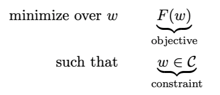
其中C⊂Rd, F:Rd→R。C是convex set,F是convex function
Convex Function和Convex set的定义
Convex Function定义

Convex Set定义

Convex Function的例子
l2-norm
F(w)=∥x∥22=x⊤x
Logistic
F(w;x,y)=log(1+exp(−yw⊤x))
Mean of Convex Functions
F(w)=m1i=1∑mFi(w)
Convex Function的first and second order
可以用这俩来判断是不是convex function,其中second order最常用
First Order
for all$ \omega, \omega’ \in \mathbb{R}^d, $
F(ω′)≥F(ω)+∇F(ω)⊤(ω′−ω)
解释:该函数在任何一点上都位于切线之上
Second Order(常用于判断是不是convex function)
for all ω∈Rd,
∇2F(ω)⪰0
或者说Hessian矩阵∇2F(ω)是 semi-definite (PSD)的
解释:函数的曲率总是非负的
Theorm定理
当w满足∇F(ω)=0的时候,w是F的global minimum
证明:
F(w′)≥F(w)+∇F(w)⊤(w′−w)⇒F(w′)≥F(w)
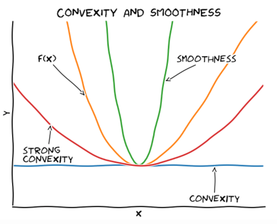
Convex Function的三条bound
-
L-smooth Function (upper bound)
For all w,w′∈Rd
F(w′)≤F(w)+∇F(w)⊤(w′−w)+2L∥w−w′∥22
-
Convex Function (lower bound)
For all w,w′∈Rd
F(w′)≥F(w)+∇F(w)⊤(w′−w)
-
μ - Strong Convex Function (lower bound)
For all w,w′∈Rd
F(w′)≥F(w)+∇F(w)⊤(w′−w)+2μ∥w−w′∥22
Gradient Descent
算法本身(GD)
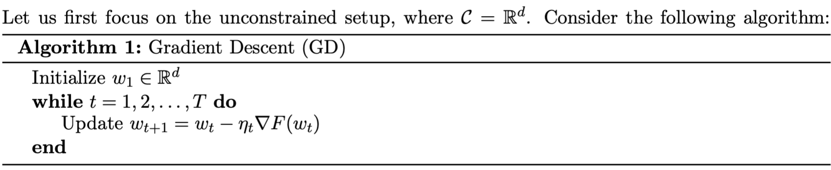
其中ηt叫做learning rate,表示每次移动多元。其中stopping condition我们一般设置为F(ωt)≤ϵ或者∥∇F(ωt)∥2≤ϵ
选择Learning Rate / Step Size
过大的learning rate会使得结果diverge,甚至会产生negative progress
过小的learning rate会会需要花费很多时间才能converge
Gradient Descent for Smooth Functions
L-Smoothness Function
for all$ \omega, \omega’ \in \mathbb{R}^d $,
F(w′)≤F(w)+∇F(w)⊤(w′−w)+2L∥w−w′∥22
等价于说∇F是L-Lipschitz
∥∇F(w)−∇F(w′)∥2≤L∥w−w′∥2
用smoothness对gradient descent进行解释
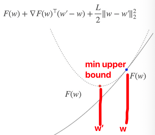
为了minF at w,我们选择min upper bound(L-smoothness),也就是下面这个式子
w′minF(w)+∇F(w)⊤(w′−w)+2L∥w′−w∥22
通过令导数等于0,我们可以求出下一步的w即w’
w′=w−L1∇F(w)
通过对比算法GD,我们可以看出来这就是gradient step with learning rate$ η = 1/L $的时候
即根据upper bound,我们求upper bound min的时候算出来的w’所对应的是upper bound的最低点,其对应的F(w’)一定比F(w)小,从而实现gradient descent
Converge的证明
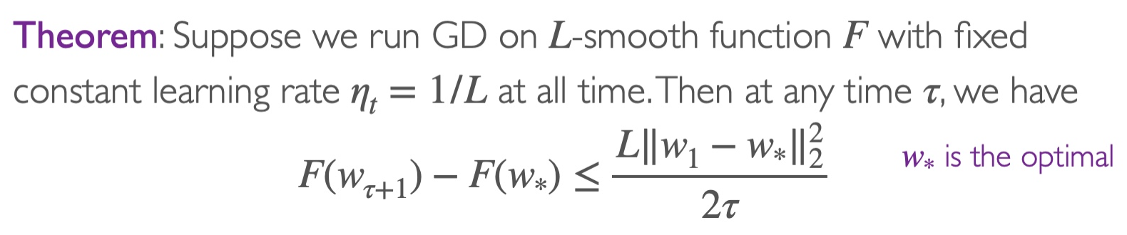
定理
解释
假设开始的时候w1=0且∥ω∗∥2=1,则在T iterations之后可以得到
F(wT+1)−F(ω∗)≤2TL
这表示了在T=2ϵL=O(1/ϵ) step之后,我们可以得到F(wT+1)−F(w∗)≤ϵ。所以我们说gradient descent has a convergence rate of O(1/T)
证明
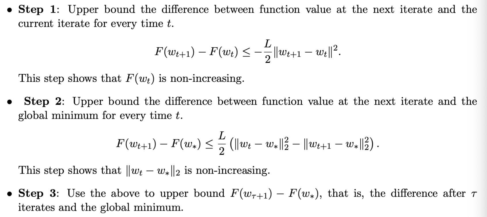
具体证明见pdf(Lec10-2)
Gradient Descent on Smooth and Strongly Convex Functions
μ- Strongly Convex Function
for all$ \omega, \omega’ \in \mathbb{R}^d $,
F(w)的lower bound
F(w′)≥F(w)+∇F(w)⊤(w′−w)+2μ∥w−w′∥22
Converge证明
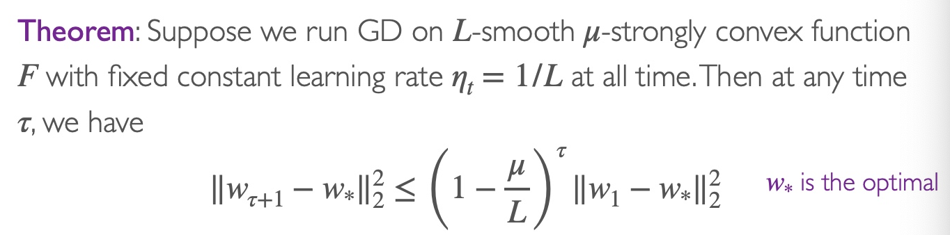
定理
解释
假设开始的时候w1=0且∥ω∗∥2=1,则在T iterations之后可以得到
∥wT+1−w∗∥22≤(1−Lμ)⊤
这表示了在T=μLlog(1/ϵ)=O(log(1/ϵ)) step之后,我们可以得到∥wT+1−w∗∥2≤ϵ。所以我们说gradient descent has a convergence rate of O(exp(−T))
附录
GD converge with L smooth和F的证明
Step1
根据smoothness的式子1,我们可以知道在t时刻
F(wt+1)−F(wt)≤∇F(wt)⊤(wt+1−wt)+2L∥wt+1−wt∥22
将∇F(wt)=L(wt−wt+1)带入式(4)
F(wt+1)−F(wt)≤L(wt−wt+1)⊤(wt+1−wt)+2L∥wt+1−wt∥22=−L(wt+1−wt)⊤(wt+1−wt)+2L∥wt+1−wt∥22=−L∥wt+1−wt∥22+2L∥wt+1−wt∥22=−2L∥wt+1−wt∥22
Step2
根据convex function的式子2和∇F(wt)=L(wt−wt+1),我们可以得到
F(w∗)⇒F(wt)−F(w∗)≥F(w)+∇F(w)⊤(w∗−w)≤L(wt−wt−1)⊤(wt−w∗)
又因为
∥wt+1−w∗∥22=∥wt+1−wt+wt−w∗∥22=∥wt+1−wt∥22+∥wt−w∗∥22+2(wt+1−wt)⊤(wt−w∗)
将式子(7)带入式子(6),我们可以得到
F(wt)−F(w∗)≤2L(∥wt+1−wt∥22+∥wt−w∗∥22−∥wt+1−w∗∥22)
将式子(5)带入式子(8)
F(wt+1)−F(wt)+F(wt)−F(w∗)F(wt+1)−F(w∗)≤2L(∥wt+1−wt∥22+∥wt−w∗∥22−∥wt+1−w∗∥22)+(−2L∥wt+1−wt∥22)≤2L(∥wt−w∗∥22−∥wt+1−w∗∥22)
Step3
根据式9,从tau+1累加到tau可以得到下式
F(wτ+1)−F(w∗)+F(wτ+1)−F(w∗)+...+F(wτ+1)−F(w∗)=τ(F(wτ+1)−F(w∗))≤F(wτ+1)−F(w∗)+F(wτ)−F(w∗)+...+F(w1)−F(w∗)=t=1∑τ(F(wt+1)−F(w∗))≤2L(∥wτ−w∗∥22−∥wτ+1−w∗∥22+∥wτ−1−w∗∥22−∥wτ−w∗∥22)+...+∥w1−w∗∥22−∥w2−w∗∥22)≤2L(∥w1−w∗∥22−∥wτ+1−w∗∥22)≤2L∥w1−w∗∥22
带入w1=0和∥w∗∥22=1,可以求出来经过T次迭代之后(即τ=T),
F(wT+1)−F(w∗)≤2TL
这表示经过T=2ϵL次迭代,函数F收敛,即F(wT+1)−F(w∗)≤ϵ
不同梯度下降算法的比较(非课程要求)
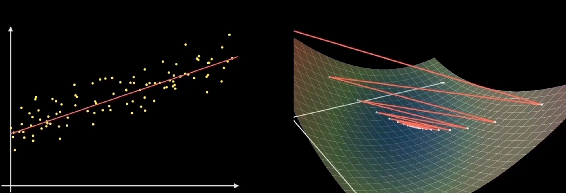
批量梯度下降|标准梯度下降|Batch GD
每次使用所有的样本进行计算梯度(i=1~n)
f(x)=n1i=1∑nfi(x)∇f(x)=n1i=1∑n∇fi(x)
优点:梯度更新准确
缺点:只有convex function才可以保证最后得到的是全剧最优;收敛速度很慢
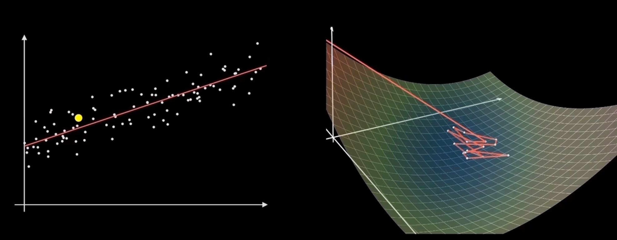
随机梯度下降|Stochastic GD
每次下降只用一个样本点进行计算(i是1-n的任意值,随机选取的样本点)
f(x)=fi(x)∇f(x)=∇fi(x)
优点:训练速度快
缺点:容易在最优的地方反复横跳而到不了最优点,只能在最优点周围
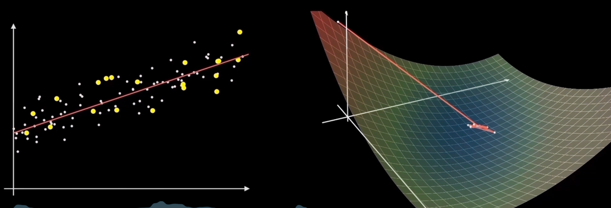
小批量梯度下降|Mini-Batch GD
每次下降选用一批样本点进行计算(从n个样本点里面随机选取k个样本)
f(x)=k1i=1∑kfi(x)∇f(x)=k1i=1∑k∇fi(x)
优点:训练速度快
缺点:选择平均梯度最小的方向
声明:此blog内容为上课笔记,仅为分享使用。部分图片和内容取材于课本、老师课件、网络。如果有侵权,请联系aursus.blog@gmail.com删除。