Binary Classification
假设
- 可线性分割的数据
- Binary classification,即数据是可以分为两类的
目的
将数据按照label分为两个类别
Set up
input space
X=Rd
label space / output space
Y={−1,1}
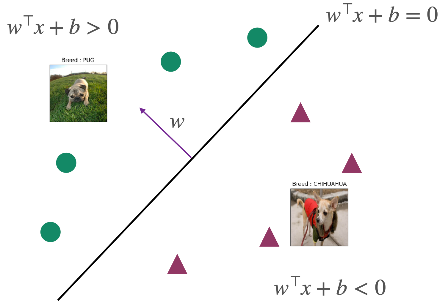
分类器|classifier|hypothesis class F
F:={x↦sign(w⊤x+b) ∣ w∈Rd,b∈R}
其中ω是weight vector;b是bias,sign是符号函数,具体定义如下:
sign(a)={1−1if a≥0otherwise
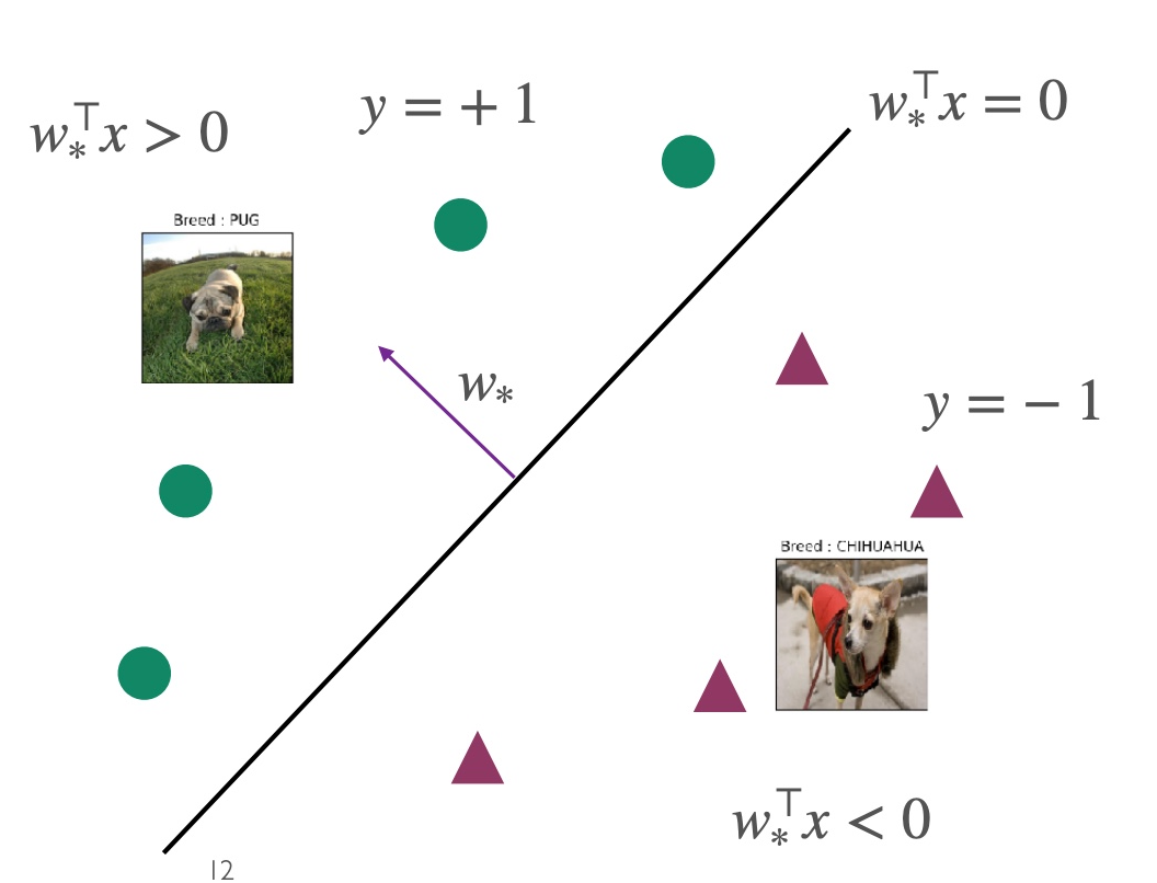
为了简化后续的计算,我们希望classifier只含有w但没有b,因此我们通过增加一个维度,将b放在w的第二个维度作为常数看待,具体如下:
x↦[x1]w↦[wb]
原始classifier简化为
F:={x↦sign(w⊤x) }
Empricial Risk Minizer
我们使用如下的loss function来求ERM
ℓ(f(x),y)={01if f(x)=yotherwise
该式子也被称为0-1 loss,1代表预测错误,0代表预测正确。该式子也可以用指示函数I(Indicator function)表示:
I[f(x)=y]={10if f(x)=yif f(x)=y
通过将classifier带入loss function,可以求出ERM如下
wminerr^(w)=wminm1i=1∑mI[sign(w⊤xi)=yi]=wminm1i=1∑mI[sign(yiw⊤xi<0)]
能够使ERM最小的w被称为w^:
w^=argwminm1i=1∑mI[sign(w⊤xi)=yi]=argwminm1i=1∑mI[sign(yiw⊤xi<0)]
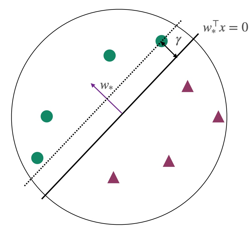
当数据集是线性可分割的,则w^被称为w∗,此时的w∗对任意点而言,均满足yi=sign(ω∗⊤xi),且此时的ω∗⊤xi是两种类别的分界线
Perceptron 算法
目的
更新w直到所有数据点都能正确分类
适用范围
- 数据点要求完全线性可分割
- 一旦出现类似XOR的数据或者线性不可分割(Non-linearly separable data)的数据,则无法使用perceptron
- XOR和Non-linearly的数据可以用kernel SVM分割
算法
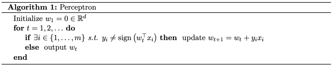
更新规则
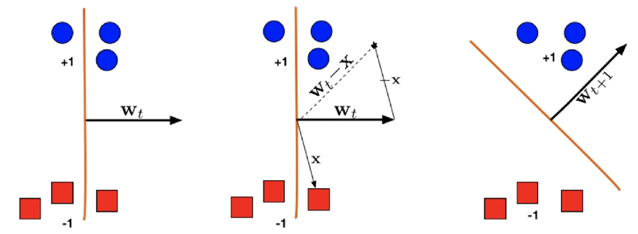
如果分类错误,即sign(w⊤xi)=yi或者sign(yiw⊤xi<0),则按照规则wt+1=wt+yixi进行更新
如果yi=1则wt+1⊤xi=wt⊤xi+∥xi∥2>wt⊤xi,w向着positive的方向更新
如果yi=−1则wt+1⊤xi=wt⊤xi−∥xi∥2<wt⊤xi,w向着negative的方向更新
margin γ 和算法收敛Convergence
前提条件:所有点都在单位圆内∣∣xi∣∣2≤1,并且此时的∣∣ω∗∣∣=1
结论:Perceptron algorithm至多进行1/γ2轮就会收敛,且会返回sign(ωTxi)=yi的分类器,此时所有点都被正确分类
证明:参考https://machine-learning-upenn.github.io/assets/notes/Lec2.pdf
**margin γ **:表示所有点到超平面(hyperplane)的最小距离
γ=i∈[m]min∥w∥∣w∗⊤xi∣=i∈[m]min∣w∗⊤xi∣
reference:
https://www.cs.cornell.edu/courses/cs4780/2022sp/notes/LectureNotes06.html
https://machine-learning-upenn.github.io/calendar/
声明:此blog内容为上课笔记,仅为分享使用。部分图片和内容取材于课本、老师课件、网络。如果有侵权,请联系aursus.blog@gmail.com删除。