BME | Machine Learning - Logistic Regression
Logistic Regression
Utilization: Curve fitting, classification into two classes, typically deals with data points.
Applicability: Can be applied universally. If data separation can be achieved with a single line, logistic regression can be used.
Input Space
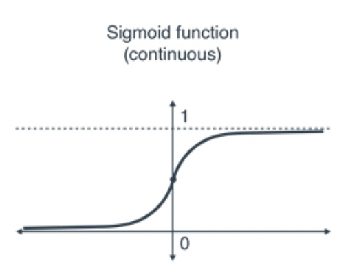
Label Space/Output Space (y ranges from 0 to 1)
Hypothesis Class
Note: : weight vector; : bias
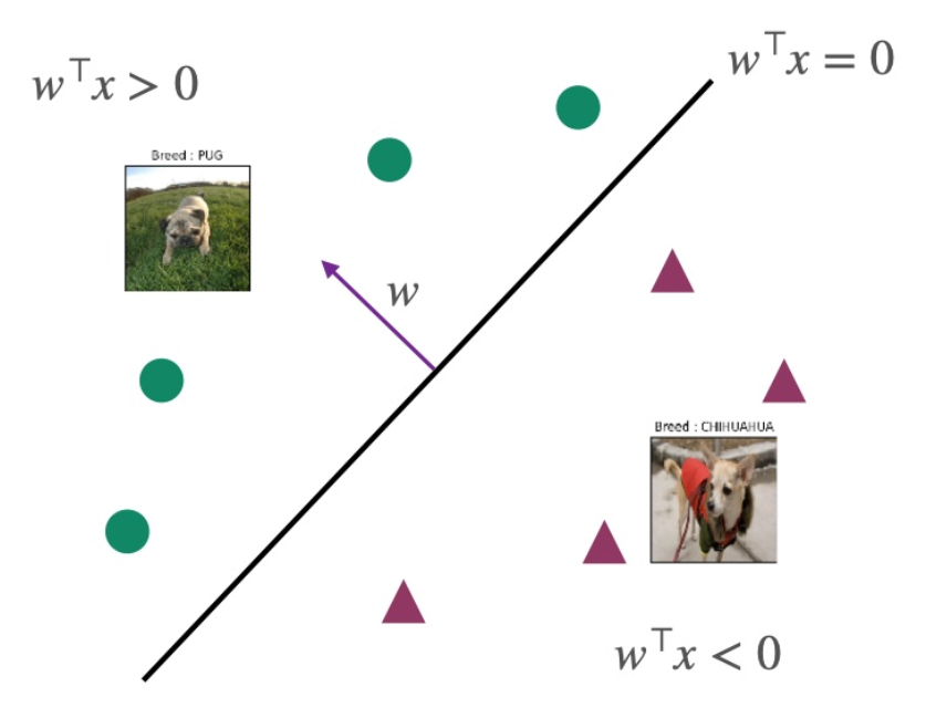
Decision Boundary
The result of indicates:
- If , then .
- If , then , indicating a higher probability for label=1.
- If , then , indicating a higher probability for label=-1.
- If , then , precisely at the decision boundary.
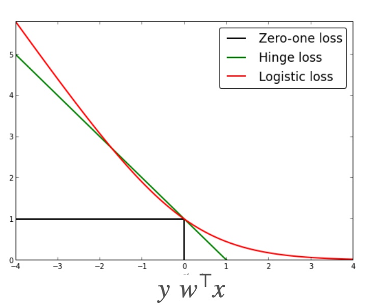
Loss Function (Derivation of ERM - Method 1)
Substituting and simplifying yields .
Note: This is the logistic loss, where 1 represents a wrong prediction and 0 indicates a correct prediction.
MAXIMUM LIKELIHOOD ESTIMATOR (Derivation of ERM - Method 2)
Objective: To achieve optimal results, it can be compared to the loss function where one maximizes probability and the other minimizes error.
Bayesian distribution, the product of probabilities of all and given the parameter .
represents the train data. ERM can be derived from the above equation by taking its logarithm. For specific derivation steps, refer to the slides.
Empirical Risk Minimizer (Convex)
Disclaimer: This blog content is intended as class notes and is solely for sharing purposes. Some images and content are sourced from textbooks, teacher presentations, and the internet. If there are any copyright infringements, please contact aursus.blog@gmail.com for removal.