Concept
Purpose: Dimensionality Reduction
input x⊂Rd, {x(i);i=1,...,n}
output Z⊂Rk
F:X→Z, k<<d
Here, i denotes the number of samples (total n), and j denotes the number of features (total d).
Preprocessing|Data Preprocessing
Purpose: Normalize all features to data with mean=E[xj(i)]=0 and variance=Var[xj(i)]=1
Method:
xj(i)←σjxj(i)−μjwhere, μj=n1i=1∑nxj(i), σj2=n1i=1∑n(xj(i)−μj)2
If we can ensure that different features have the same scale, it can be represented as:
? Parameter estimation utilizes the EM algorithm
Computing Major Axis of Variation u
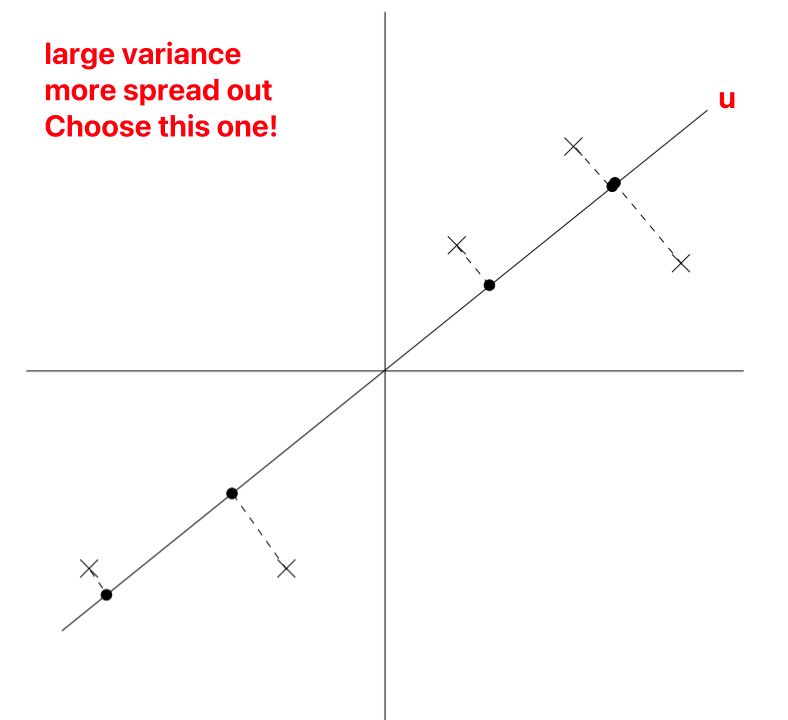

u is a unit vector, x represents the sample, denoted as different points on the graph.
During projection (reducing 2D to 1D), to retain more information, we choose the projection data’s variance, i.e., the projection points’ distribution that is more uniform.
As normalization has been performed, u must necessarily pass through the origin.
Maximizing Projection Variance
The projection of point x onto vector u is xTu,
Calculation of Projection:
∣∣Proju(x)∣∣2=∣xTu∣
Calculation of Variance:
Var(Proju(x))=∣xTu∣2
Variance of all points x projected onto a single u:
n1i=1∑n(x(i)Tu)2=n1i=1∑nuTx(i)x(i)Tu=uT(n1i=1∑nx(i)x(i)T)u=uTΣ^u
If ∣∣u∣∣2=1, the principal eigenvector can be simplified as Σ^=n1∑i=1nx(i)x(i)T, i.e.,
∣∣u∣∣2=1maxuTΣ^u=λ1
Where λ_1 represents the first eigenvalue of Σ^ (principal eigenvalues), and in this case, u represents the 1st principal eigenvector of Σ^.
Summary
The best 1D direction for x is the 1st eigenvector of covariance, i.e., v1Σˉ. PyTorch’s torch.lobpcg function can be utilized.
If we want to project data to 1D, select u to be the principal eigenvector of Σ.
Projected data after reducing dimensions: X.mm(V), where V represents the first k eigenvectors, with size (d, k). Here, X goes from m×d dimensions to m×k.
If we aim to project data into k dimensions:
Method 1: Choose u1,u2,...,uk to be the top k eigenvectors of Σ.
u1,u2,...,ukmaxi=1∑u∣∣∣∣∣∣∣∣∣∣∣∣∣∣∣∣∣∣⎣⎢⎢⎢⎡u1Tx(i)u2Tx(i)...ukTx(i)⎦⎥⎥⎥⎤∣∣∣∣∣∣∣∣∣∣∣∣∣∣∣∣∣∣22=v1,v2,...,vk
Method 2:
u1,u2,...,ukmini=1∑n∣∣xi−xˉi∣∣22=i=1∑n∣∣xi−l=1∑k(ulTxi)ul∣∣22
Here, xˉi represents the reconstruction example given by basic components.
Note: The content in this blog is class notes shared for educational purposes only. Some images and content are sourced from textbooks, teacher materials, and the internet. If there is any infringement, please contact aursus.blog@gmail.com for removal.