BME | EEG Analysis - Hilbert Transform
Hilbert Transform | Hilbert Transform
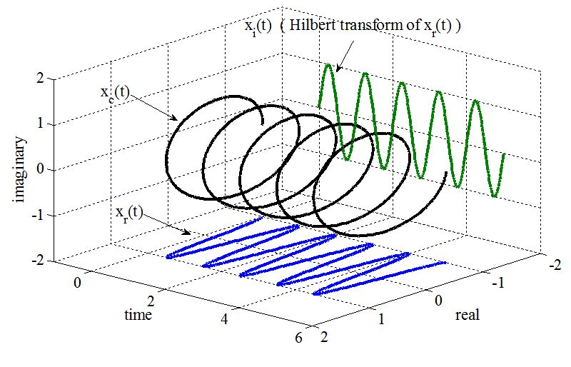
Basic procedure: Start with a bandpass filter, then apply the Hilbert transform to obtain a complex signal, which separates amplitude and phase.
Objective: Obtain instantaneous amplitude and phase by adding the imaginary part to the real signal.
📌 We do not alter the real part; we only add the imaginary part on top of it.
Mathematical Definition
Assuming we have a signal named , the Hilbert transform is given by:
The imag signal is the result of shifting the real signal by . For example, if the original signal is , then the result after the Hilbert transform will be .
Code
MATLAB Code
1 | % Hilbert Custom function |
1 | % using Hilbert function |
Python Code
1 | # Hilbert Custom function |
1 | # using Hilbert function |
Filtering | Filter
Filtering the data before applying the Hilbert transform is crucial to prevent wide bandwidths that could lead to challenging interpretations.
Two common types of filters: Finite Impulse Response (FIR) and Infinite Impulse Response (IIR).
Advantages and characteristics of FIR compared to IIR:
- FIR kernel functions are zero at positive and negative infinity.
- Wavelets can be considered a type of FIR filter.
- FIR is recommended over IIR because it’s stable and less prone to introducing nonlinear phase distortions.
- However, FIR filters are more computationally expensive.
Things to consider when designing filters:
- Sharp edges in the filter’s frequency response can cause ripples in the time domain. Thus, it’s best to design filters that are plateau-shaped and ensure transition zones cover 10% to 25% of the frequency range (max frequency - min frequency).
Code
MATLAB Code
The most common functions are firls and fir1, along with other functions available.
firls: Least-squares linear-phase FIR filter.
1 | b = firls(n, f, a) |
n: The n denotes the filter order, and the corresponding kernel length is n+1 (referring to the number of points rather than time). n has no upper limit, but higher values increase computational load. The lower limit of n ranges from 2-5 times the lowest frequency (for instance, if the lowest frequency is 10Hz, a kernel corresponding to a time length of 200-500ms is typically used).
f: f represents the x-coordinates of the filter points, indicating the scaled relative values of the filter points’ frequencies after scaling (such that Nyquist frequency = 1). For example, f = [0, 0.1, 0.15, 0.3, 0.35, 1];
a: a signifies the y-coordinates of the filter points and is scaled to the range [0,1]. For instance, a = [0 0 1 1 0 0]; Note that the lengths of a and f should be the same.
: Window-based FIR filter.
Python
Continued.
Note: The content in this blog is class notes shared for educational purposes only. Some images and content are sourced from textbooks, teacher materials, and the internet. If there is any infringement, please contact aursus.blog@gmail.com for removal.